Inverse Gaussian distribution
| Probability density function |
|
| Parameters |   |
|---|---|
| Support |  |
![\left[\frac{\lambda}{2 \pi x^3}\right]^{1/2} \exp{\frac{-\lambda (x-\mu)^2}{2 \mu^2 x}}](/2012-wikipedia_en_all_nopic_01_2012/I/2c6c7ef1a504f4998fe143af8151a018.png) |
|
| CDF | 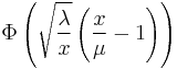 
where |
| Mean |  |
| Mode | ![\mu\left[\left(1%2B\frac{9 \mu^2}{4 \lambda^2}\right)^\frac{1}{2}-\frac{3 \mu}{2 \lambda}\right]](/2012-wikipedia_en_all_nopic_01_2012/I/d50e806b11641fa78d3ddc5f7cbc0c0b.png) |
| Variance |  |
| Skewness |  |
| Ex. kurtosis |  |
| MGF | ![e^{\left(\frac{\lambda}{\mu}\right)\left[1-\sqrt{1-\frac{2\mu^2t}{\lambda}}\right]}](/2012-wikipedia_en_all_nopic_01_2012/I/dfb098ca17eedc92acafed44a7d67d8e.png) |
| CF | ![e^{\left(\frac{\lambda}{\mu}\right)\left[1-\sqrt{1-\frac{2\mu^2\mathrm{i}t}{\lambda}}\right]}](/2012-wikipedia_en_all_nopic_01_2012/I/6bbfc39a08f359b23390648366ec800d.png) |
 is the
 In probability theory, the inverse Gaussian distribution (also known as the Wald distribution) is a two-parameter family of continuous probability distributions with support on (0,∞).
Its probability density function is given by
![f(x;\mu,\lambda)
= \left[\frac{\lambda}{2 \pi x^3}\right]^{1/2} \exp{\frac{-\lambda (x-\mu)^2}{2 \mu^2 x}}](/2012-wikipedia_en_all_nopic_01_2012/I/14b32d96e7fcbbd2b08cab10865aa654.png)
for x > 0, where is the mean and is the shape parameter.
As λ tends to infinity, the inverse Gaussian distribution becomes more like a normal (Gaussian) distribution. The inverse Gaussian distribution has several properties analogous to a Gaussian distribution. The name can be misleading: it is an "inverse" only in that, while the Gaussian describes a Brownian Motion's level at a fixed time, the inverse Gaussian describes the distribution of the time a Brownian Motion with positive drift takes to reach a fixed positive level.
Its cumulant generating function (logarithm of the characteristic function) is the inverse of the cumulant generating function of a Gaussian random variable.
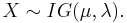
To indicate that a random variable X is inverse Gaussian-distributed with mean μ and shape parameter λ we write
Contents |
Properties
Summation
If Xi has a IG(μ0wi, λ0wi2) distribution for i = 1, 2, ..., n and all Xi are independent, then
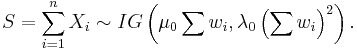
Note that
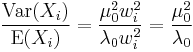
is constant for all i. This is a necessary condition for the summation. Otherwise S would not be inverse Gaussian.
Scaling
For any t > 0 it holds that

Exponential family
The inverse Gaussian distribution is a two-parameter exponential family with natural parameters -λ/(2μ²) and -λ/2, and natural statistics X and 1/X.
Relationship with Brownian motion
The stochastic process Xt given by

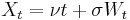
(where Wt is a standard Brownian motion and  ) is a Brownian motion with drift ν.
Then, the first passage time for a fixed level  by Xt is distributed according to an inverse-gaussian:

When drift is zero
A common special case of the above arises when the Brownian motion has no drift. In that case, parameter μ tends to infinity, and the first passage time for fixed level α has probability density function
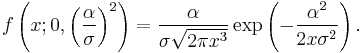
This is a Lévy distribution with parameter  .
.
Maximum likelihood
The model where

with all wi known, (μ, λ) unknown and all Xi independent has the following likelihood function

Solving the likelihood equation yields the following maximum likelihood estimates
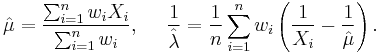
 and
and  are independent and
Generating random variates from an inverse-Gaussian distribution
The following algorithm may be used.[1]
Generate a random variate from a normal distribution with a mean of 0 and 1 standard deviation
Square the value

and use this relation
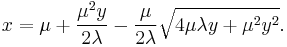
Generate another random variate, this time sampled from a uniformed distribution between 0 and 1
If

then return

else return

Sample code in Java:
public double inverseGaussian(double mu, double lambda) {
       Random rand = new Random();
       double v = rand.nextGaussian();   // sample from a normal distribution with a mean of 0 and 1 standard deviation
       double y = v*v;
       double x = mu + (mu*mu*y)/(2*lambda) - (mu/(2*lambda)) * Math.sqrt(4*mu*lambda*y + mu*mu*y*y);
       double test = rand.nextDouble();  // sample from a uniform distribution between 0 and 1
       if (test <= (mu)/(mu + x))
              return x;
       else
              return (mu*mu)/x;
}
Related distributions
- If
 then
then 
- If
 then
then 
- If for
 then
then 
- If
 then
then 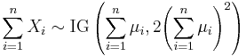
See also
Notes
- ^ Generating Random Variates Using Transformations with Multiple Roots by John R. Michael, William R. Schucany and Roy W. Haas, American Statistician, Vol. 30, No. 2 (May, 1976), pp. 88–90
References
- The inverse gaussian distribution: theory, methodology, and applications by Raj Chhikara and Leroy Folks, 1989 ISBN 0-8247-7997-5
- System Reliability Theory by Marvin Rausand and Arnljot Høyland
- The Inverse Gaussian Distribution by Dr. V. Seshadri, Oxford Univ Press, 1993
External links
- Inverse Gaussian Distribution in Wolfram website.